Tutorial to the anomaly vegetation change detection: “AVOCADO”
Introduction
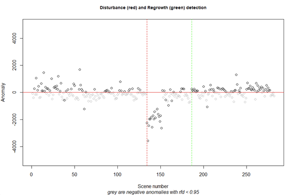
The “AVOCADO” (Anomaly Vegetation Change Detection) algorithm is a continuous vegetation change detection method that also capture regrowth. It is based on the R package “npphen” (Chavez et al., 2017), developed to monitor changes in phenology, and adjusted to monitor forest disturbance and regrowth in a semi-automated and continuous way. The algorithm uses all available data and does not require certain pre-processing steps such as removing outliers. The reference vegetation (undisturbed forest in this case) is taken from nearby pixels that are known to be undisturbed during the whole time-series, so there is no need to set aside part of the time-series as an historical baseline. By using the complete time-series in AVOCADO, more robust predictions of vegetation changes can be made while improving our ability to deal with gaps in the data. The algorithm accounts for the natural variability of the annual phenology (using the flexibility of kernel fitting), which makes it suitable to monitor areas with strong seasonality (e.g. dry ecosystems) and gradual/small changes (i.e. degradation).
More details can be found in the following paper: Decuyper, M., Chávez, R.O., Lohbeck, M., Lastra, J.A., Tsendbazar, N., Hackländer, J., Herold, M., Vågen, T.-G., 2022. Continuous monitoring of forest change dynamics with satellite time series. Remote Sens. Environ. 269, 112829. https://doi.org/https://doi.org/10.1016/j.rse.2021.112829
Step 1: Installing the required packages
The package is available through the github and can be installed via “remotes”:
library(remotes)
install_github('MDecuy/AVOCADO')
#load library
library(AVOCADO)
Please note that an explanation on all parameters of the AVOCADO algorithm can be found in the github documentation.
Other packages that are needed: rgdal, raster, npphen, bfastSpatial, RColorBrewer, rts, lubridate
Step 2: Downloading the satellite data
Currently there are various satellite sources and ways to download the data such as the Earth Explorer or the Google Earth Engine platform. There is a lot information on how to download various satellite data on the Google Earth Engine Guides platform, but here we provide a small example script for Landsat Collection 2 Level 2 data.
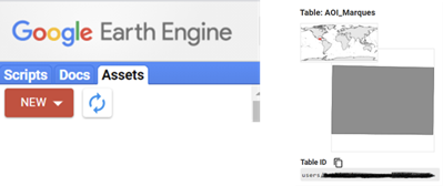
The first step is to upload the shapefile for your area of interest (AOI). This can be done under the tab “Assets” and once it is uploaded you can add the directory (see “Table ID”) into the script below (under “var input_polygon”).Show GEE code
//Downloading Landsat data via the Google Earth Engine (GEE) platform.
////////////////////////////////////////////////////////////////////////////////////
// Paste this code into your GEE script page
////////////////////////////////////////////////////////////////////////////////////
// Specify the location of the before uploaded shapefile in your assets
var input_polygon = 'users/yourusername/ AOI';
// Export folder in your google drive
var input_export_folder = 'FolderName_You_Created_in_Your_GoogleDrive_Account';
// Start and end dates
var input_StartStr = ee.String('1990-01-01');
var input_FinishStr = ee.String('2015-01-01');
/* available indices: NDVI (ndvi_ind), NBR (nbr_ind), EVI (evi_ind), SAVI (savi_ind), tasseled cap
brightness (Tcap_bri_ind), tasseled cap greenness (Tcap_gre_ind), tasseled cap wetness (Tcap_wet_ind)
Specify the vegetation indices you are interested in by marking it as TRUE, or if not as FALSE.
In this example we use NDMI.*/
var ndvi_ind = ['FALSE'];
var ndmi_ind = ['TRUE'];
var nbr_ind = ['FALSE'];
var evi_ind = ['FALSE'];
var savi_ind = ['FALSE'];
var Tcap_bri_ind = ['FALSE'];
var Tcap_gre_ind = ['FALSE'];
var Tcap_wet_ind = ['FALSE'];
///////////////////////////////////////////////////////////////////////////////////////
// END of input variables.
////////////////////////////////////////////
/* The following lines can be left default, unless you want
to change e.g. the cloud cover percentage.*/
///////////////////////////////////////////////////////////////////////////////////////
// Buffer to download around the above area, use 0 for no buffer
var input_buffer = 0;
// Convert text string dates to date tpe
var Start = ee.Date(input_StartStr);
var Finish = ee.Date(input_FinishStr);
// Create a feature collection out of the fustion table id
var Polygon = ee.FeatureCollection(ee.String(input_polygon));
// Buffer the area of interest
var PolygonBuffer = input_buffer === 0 ? Polygon.first().geometry() : Polygon.first().geometry().buffer(input_buffer);
Map.addLayer(PolygonBuffer,null,'Buffer');
Map.centerObject(PolygonBuffer);
// Standard names to rename the bands regardless of collection
var selected_bands = ['blue','green','red','nir','swir','swir2','QA_PIXEL'];
// Applies scaling factors.
var applyScaleFactors = function (image) {
var opticalBands = image.select('SR_.*').multiply(0.0000275).add(-0.2);
return image.addBands(opticalBands, null, true);
;
}
// Merge the 3 collections, select, and rename the bands to standard names
var Collection = ee.ImageCollection('LANDSAT/LT05/C02/T1_L2').map(applyScaleFactors)
.select(['SR_B1','SR_B2','SR_B3','SR_B4','SR_B5','SR_B7','QA_PIXEL'],selected_bands)
.merge(ee.ImageCollection('LANDSAT/LE07/C02/T1_L2').map(applyScaleFactors)
.select(['SR_B1','SR_B2','SR_B3','SR_B4','SR_B5','SR_B7','QA_PIXEL'],selected_bands))
.merge(ee.ImageCollection('LANDSAT/LC08/C02/T1_L2').map(applyScaleFactors)
.select(['SR_B2','SR_B3','SR_B4','SR_B5','SR_B6','SR_B7','QA_PIXEL'],selected_bands))
.sort("system:time_start") // Sort by Date
.filterDate(Start,Finish) // Filter by date
.filterBounds(PolygonBuffer) // Filter by area
.filterMetadata("CLOUD_COVER","less_than",70) // Filter by cloud cover
.map(function(image) {return image.mask(image.select('QA_PIXEL')
.remap([1,5440,21824],[1,1,1],0) // 1...21824 -> 1 = not masked
;
)//.clip(PolygonBuffer)
};
)
print('Collection of Landsat Scenes',Collection);
// Mosaicking by day
// Create list with dates
var Days = Finish.difference(Start, 'day')
var Dates = ee.List.sequence(0, Days.subtract(1)).map(function(Day){return Start.advance(Day,'day')})
// Function that does day mosaicking
var day_mosaicking = function day_mosaicking(date, newlist) {
// Cast
= ee.Date(date)
date = ee.List(newlist)
newlist
// Filter collection between date and the next day
var filtered = Collection.filterDate(date, date.advance(1,'day'));
var first = filtered.first();
// Make the mosaic
var image = ee.Image(filtered.mosaic())
= image.set('system:time_start',date.millis());
image = image.set('SATELLITE',first.get('SATELLITE'));
image // Add the mosaic to a list only if the collection has images
return ee.List(ee.Algorithms.If(filtered.size(), newlist.add(image), newlist))
}// Iterate through dates and create a collection with mosaicked images
= ee.ImageCollection(ee.List(Dates.iterate(day_mosaicking, ee.List([]))))
Collection
// Calculate the normalized difference index (ndi), give it a name and merge all single band images
var mergeBands = function mergeBands(image, previous) {
return ee.Image(previous).addBands(image);
;
}
// NDVI calculation
if (ndvi_ind == 'TRUE'){
var input_index = "NDVI"
var index_bands = ['nir','red'];
var NDVI = Collection
.map(function(image) {return image.normalizedDifference(index_bands)
.rename(ee.String(input_index+'_').cat(image.get('SATELLITE'))
.cat('_')
.cat(ee.Date(image.get('system:time_start')).format('YYYYMMdd')))
}).iterate(mergeBands, ee.Image([]));
var NDVI = ee.Image(NDVI).multiply(ee.Image(10000))
.round()
.toFloat()
.clip(PolygonBuffer);
.image.toDrive({
Exportimage:NDVI,
description: 'Landsat_' + input_index + '_' + input_StartStr.getInfo() + '_' + input_FinishStr.getInfo(),
folder: input_export_folder,
region: PolygonBuffer,
scale: 30,
maxPixels: 10e10
})
}
// NDMI calculation
if (ndmi_ind == 'TRUE'){
var input_index = "NDMI"
var index_bands = ['nir','swir'];
var NDMI = Collection
.map(function(image) {return image.normalizedDifference(index_bands)
.rename(ee.String(input_index+'_').cat(image.get('SATELLITE'))
.cat('_')
.cat(ee.Date(image.get('system:time_start')).format('YYYYMMdd')))
}).iterate(mergeBands, ee.Image([]));
var NDMI = ee.Image(NDMI).multiply(ee.Image(10000))
.round()
.toFloat() //change this to avoid zero values
.clip(PolygonBuffer);
// (iv) extracting the band layer names for dates to export a table of the dates
var asList = NDMI.bandNames().map(function (layer) {
return ee.Feature(null, {Date: ee.String(layer)});
;
})var feature_date = ee.FeatureCollection(asList);
.image.toDrive({
Exportimage:NDMI,
description: 'Landsat_' + input_index + '_' + input_StartStr.getInfo() + '_' + input_FinishStr.getInfo(),
folder: input_export_folder,
region: PolygonBuffer,
scale: 30,
maxPixels: 10e10
})
.table.toDrive({
Exportcollection:feature_date,
description: 'Date_Landsat_' + input_index + '_' + input_StartStr.getInfo() + '_' + input_FinishStr.getInfo(),
folder: input_export_folder
})
}
// NBR calculation
if (nbr_ind == 'TRUE'){
var input_index = "NBR"
var index_bands = ['nir','swir'];
var NBR = Collection
.map(function(image) {return image.normalizedDifference(index_bands)
.rename(ee.String(input_index+'_').cat(image.get('SATELLITE'))
.cat('_')
.cat(ee.Date(image.get('system:time_start')).format('YYYYMMdd')))
}).iterate(mergeBands, ee.Image([]));
var NBR = ee.Image(NBR).multiply(ee.Image(10000))
.round()
.toFloat()
.clip(PolygonBuffer);
.image.toDrive({
Exportimage:NBR,
description: 'Landsat_' + input_index + '_' + input_StartStr.getInfo() + '_' + input_FinishStr.getInfo(),
folder: input_export_folder,
region: PolygonBuffer,
scale: 30,
maxPixels: 10e10
})
}
// EVI calculation
if (evi_ind == 'TRUE'){
var input_index = "EVI"
var index_bands = ['blue','red','nir'];
var EVI = Collection
.map(function(image) {return image.expression('2.5 * ((NIR - RED) / ((NIR + 6 * RED - 7.5 * BLUE) + 1))',{
'BLUE': image.select(index_bands[0]),
'RED': image.select(index_bands[1]),
'NIR': image.select(index_bands[2])
}).rename(ee.String(input_index+'_').cat(image.get('SATELLITE'))
.cat('_')
.cat(ee.Date(image.get('system:time_start')).format('YYYYMMdd')))
}).iterate(mergeBands, ee.Image([]));
var EVI = ee.Image(EVI).clip(PolygonBuffer);
.image.toDrive({
Exportimage:EVI,
description: 'Landsat_' + input_index + '_' + input_StartStr.getInfo() + '_' + input_FinishStr.getInfo(),
folder: input_export_folder,
region: PolygonBuffer,
scale: 30,
maxPixels: 10e10
})
}
//SAVI calculation
if (savi_ind == 'TRUE'){
var input_index = "SAVI"
var index_bands = ['red','nir'];
var SAVI = Collection
.map(function(image) {return image.expression('((NIR - RED) / (NIR + RED + 0.5))*(1 + 0.5)',{
'RED': image.select(index_bands[0]),
'NIR': image.select(index_bands[1])
}).rename(ee.String(input_index+'_').cat(image.get('SATELLITE'))
.cat('_')
.cat(ee.Date(image.get('system:time_start')).format('YYYYMMdd')))
}).iterate(mergeBands, ee.Image([]));
var SAVI = ee.Image(SAVI).clip(PolygonBuffer);
.image.toDrive({
Exportimage:SAVI,
description: 'Landsat_' + input_index + '_' + input_StartStr.getInfo() + '_' + input_FinishStr.getInfo(),
folder: input_export_folder,
region: PolygonBuffer,
scale: 30,
maxPixels: 10e10
})
}
// Tasselled Cap - brightness
if (Tcap_bri_ind == 'TRUE'){
var input_index = "Tcap_bright"
var index_bands = ['blue','green','red','nir','swir','swir2'];
var Tcap_bright = Collection
.map(function(image) {return image.expression('0.3037 * BLUE + 0.2793 * GREEN + 0.4743 * RED + 0.5585 * NIR + 0.5082 * SWIRI + 0.1863 * SWIRII',{
'BLUE': image.select(index_bands[0]),
'GREEN': image.select(index_bands[1]),
'RED': image.select(index_bands[2]),
'NIR': image.select(index_bands[3]),
'SWIRI': image.select(index_bands[4]),
'SWIRII': image.select(index_bands[5])
}).rename(ee.String(input_index+'_').cat(image.get('SATELLITE'))
.cat('_')
.cat(ee.Date(image.get('system:time_start')).format('YYYYMMdd')))
}).iterate(mergeBands, ee.Image([]));
var Tcap_bright = ee.Image(Tcap_bright).clip(PolygonBuffer);
.image.toDrive({
Exportimage:Tcap_bright,
description: 'Landsat_' + input_index + '_' + input_StartStr.getInfo() + '_' + input_FinishStr.getInfo(),
folder: input_export_folder,
region: PolygonBuffer,
scale: 30,
maxPixels: 10e10
})
}
// Tasselled Cap - greenness
if (Tcap_gre_ind == 'TRUE'){
var input_index = "Tcap_green"
var index_bands = ['blue','green','red','nir','swir','swir2'];
var Tcap_green = Collection
.map(function(image) {return image.expression('- 0.2848 * BLUE - 0.2435 * GREEN - 0.5436 * RED + 0.7243 * NIR + 0.0840 * SWIRI - 0.1800 * SWIRII',{
'BLUE': image.select(index_bands[0]),
'GREEN': image.select(index_bands[1]),
'RED': image.select(index_bands[2]),
'NIR': image.select(index_bands[3]),
'SWIRI': image.select(index_bands[4]),
'SWIRII': image.select(index_bands[5])
}).rename(ee.String(input_index+'_').cat(image.get('SATELLITE'))
.cat('_')
.cat(ee.Date(image.get('system:time_start')).format('YYYYMMdd')))
}).iterate(mergeBands, ee.Image([]));
var Tcap_green = ee.Image(Tcap_green).clip(PolygonBuffer);
.image.toDrive({
Exportimage:Tcap_green,
description: 'Landsat_' + input_index + '_' + input_StartStr.getInfo() + '_' + input_FinishStr.getInfo(),
folder: input_export_folder,
region: PolygonBuffer,
scale: 30,
maxPixels: 10e10
})
}
// Tasselled Cap - wetness
if (Tcap_wet_ind == 'TRUE'){
var input_index = "Tcap_wet"
var index_bands = ['blue','green','red','nir','swir','swir2'];
var Tcap_wet = Collection
.map(function(image) {return image.expression('0.1509 * BLUE + 0.1973 * GREEN + 0.3279 * RED + 0.3406 * NIR - 0.7112 * SWIRI - 0.4572 * SWIRII',{
'BLUE': image.select(index_bands[0]),
'GREEN': image.select(index_bands[1]),
'RED': image.select(index_bands[2]),
'NIR': image.select(index_bands[3]),
'SWIRI': image.select(index_bands[4]),
'SWIRII': image.select(index_bands[5])
}).rename(ee.String(input_index+'_').cat(image.get('SATELLITE'))
.cat('_').cat(ee.Date(image.get('system:time_start')).format('YYYYMMdd')))
}).iterate(mergeBands, ee.Image([]));
var Tcap_wet = ee.Image(Tcap_wet).clip(PolygonBuffer);
.image.toDrive({
Exportimage:Tcap_wet,
description: 'Landsat_' + input_index + '_' + input_StartStr.getInfo() + '_' + input_FinishStr.getInfo(),
folder: input_export_folder,
region: PolygonBuffer,
scale: 30,
maxPixels: 10e10
})
}
The AVOCADO algorithm does not require any pre-processing, but requires the dates of the raster brick in a certain format. For example, the Landsat scenes with ID “LT51970551990037” of which the last part consists of the year and julian day, needs to be converted to “1990-02-06” (these are needed to create the “lan.dates” object in step 3). The sensor name does not really matter as long as the character length stays the same. From the GEE script above you obtain a _*.tif_ file and a _*.csv_ file. Since the R software seems not to read the dates from the _*.tif_ raster brick, the dates can be extracted from the _*.csv_ file and pasted to the raster brick. Below you can find the steps in R (you can skip this step if you use the example raster stack (in step 3) provided in this tutorial:
#Loading the raster stack
<- stack("YourDirectory/data /Landsat_NDMI_2000-01-01_2021-12-31.tif")
MDD_NDMIst
#create column with Landsat scene ID for each layer
#string should be: 'LC8020049YYYYDDD' --> so each layer gets Landsat 8 assigned,
#although they might be from other satellites
#convert date column to julian days (year_month_day)
#Loading the csv file with the dates
<- read.csv("YourDirectory/data/Date_Landsat_NDMI_2000-01-01_2021-12-31.csv",
mdc_dates_raw sep=",", header=TRUE)
#Extract the dates from the text string within the csv file
<- as.character((substr(mdc_dates_raw[,2], (nchar(mdc_dates_raw[1,2])-7),
dates nchar(mdc_dates_raw[1,2]))))
#convert date column to julian days
<- data.frame(date2 = as.Date(dates, format="%Y%m%d"))
df_LSid $julian <- format(df_LSid$date2, "%Y%j")
df_LSid$id <- NA
df_LSid$id <- paste('LC8197055',df_LSid$julian, sep='')
df_LSidnames(MDD_NDMIst) <- df_LSid$id # Check the 'MDD_NDMIst' object in the R console,
#the names should look like this LC81970552021283, where 2021283 is the year and DOY.
writeRaster(MDD_NDMIst,"YourDirectory/data/Landsat_withDates_NDMI.grd", datatype="INT2S")
Please check the “getSceneinfo” function for more details and see the example output (“lan.info” and “lan.dates”) in step 3.
Step 3: Load the brick in R and create the reference phenological curve
If you are using your own data, replace accordingly.
#Loading the raster stack
<- stack(system.file("extdata", "MDD_NDMI_1990_2020.gri", package = "AVOCADO"))
MDD #Extract the dates from the brick
<- getSceneinfo(names(MDD))
lan.info #example output should look like: LT51670651984137 TM 167 65 1984-05-16
<- as.Date(lan.info$date)
lan.dates #example output should look like: "1984-05-16"
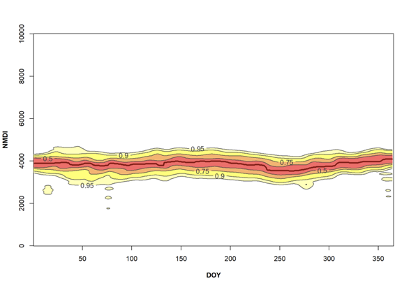
Create the vegetation reference curve (in the case of forest monitoring, this should be an area of undisturbed forest such as forest in a national park – often verified on high resolution images such as available via GEE or Google Earth Pro). It is possible to create a reference based on one pixel, but it is recommended to use several pixels (think in the range of 100-100.000 pixels) to account for natural variation between tree species.
# Load in the shapefile for the reference curve
#ref.core.shp <- readOGR(dsn=path.expand("YourDirectory/data"), layer="MDD_RefForest")
load(system.file("extdata", "MDDref.RData", package = "AVOCADO"))
#in case the coordinate between the stack and the polygon is different
#ref.core_CRS.shp <- spTransform(ref.core.shp, "+proj=longlat +datum=WGS84 +no_defs +ellps=WGS84 +towgs84=0,0,0")
To obtain a smooth reference curve, the median of the pixels per data point can be taken, but in this example we do not use this in order to take into account all the variation.
#Create the reference curve
<- extent(MDDref)
ref.ext <- crop(MDD,ref.ext)
ref.brick <- nrow(ref.brick)*ncol(ref.brick)
fin <- extract(ref.brick,1)
phen <- lan.dates
d1 for(i in 2:fin) {
<-extract(ref.brick,i)
pp <-c(phen,pp)
phen <-c(d1,lan.dates)
d1
}PhenKplot(phen, d1, h = 1, xlab = "DOY", ylab = "NDMI",rge = c(0,10000))
Step 4: Calculate the anomalies and their likelihoods
For this step you need the raster stack and the reference curve. If the site location is in the northern hemisphere use h=1 (all reference curves that look gaussian shaped or have little variation), or h=2 in the southern hemisphere (all reference curves that have a U-shape). It is very important to change anop=c(1:N) with n= number of layers in your raster stack.
Please note that this can take a few hours on one CPU, and depends on your computer properties. If you want to analyze your own (larger) area it is recommended to use a server with multiple CPU’s so you can use the multicore option, or alternatively use cloud computing services.
#checking availiable cores and leave one free
<- parallel::detectCores()-1
nc1
PlUGPhenAnoRFDMapPLUS (s = MDD,dates = lan.dates,h = 1,phen = phen,anop = c(1:1063),
nCluster = nc1, outname = "YourDirectory/MDD_AnomalyLikelihood.tif",
format = "GTiff", datatype = "INT2S", rge = c(0,10000))
# The output file contains all the anomalies, followed by all their likelihoods
# and thus has twice the number of layers as the input raster stack.
Step 5: The disturbance and regrowth detection
For this step you can set the likelihoods (rfd) and other disturbance/regrowth conditions (please visit github documentation for the details).
# Load in the anomaly and likelihood stack
<- stack("YourDirectory/MDD_AnomalyLikelihood.tif")
ano.rfd.st dist.reg.map(s = ano.rfd.st, dates = lan.dates, rfd = 0.95, dstrb_thr = 1,rgrow_thr = 730,
cdates = 3, nCluster = 1, outname = " YourDirectory/MDD_ChangeMap.tif",
format = "GTiff", datatype = "INT2S")
The output file will always contain 16 bands as shown in the figure below (Band 1: First disturbance year; Band 2: Anomalies coinciding with the first disturbance ; Band 3: First regrowth year; Band 4: Anomalies coinciding with the first regrowth; Band 5: Second disturbance year; etc.). For example: If a pixel has only values in the first 4 bands, followed by NA’s in the next bands, the pixel had only one disturbance and one regrowth event.
Reference
- Chávez, R. O., Estay, S. A., Lastra, J. A., Riquelme, C. G., Olea, M., Aguayo, J., & Decuyper, M. (2023). npphen: An R-Package for Detecting and Mapping Extreme Vegetation Anomalies Based on Remotely Sensed Phenological Variability. Remote Sensing, 15(1), 73.